Logistic Regression and Laplace's Approximation

Logistic Regression

When we train a logistic regression model, we find the maximum of the following likelihood function across the training data set (disregard regularization for now):

$$\mathcal{L}(x;\beta )=\prod _{i=1}^{n}g(x_i^{\top }\beta {)}^{y_i}\cdot (1-g(x_i^{\top }\beta ){)}^{1-y_i}$$

Here, $x_i$ represents the features of a training example, $y_i$ the label (i.e. 1 for “true”, 0 for “false”), $\beta$ the model coefficients, and $g$ the sigmoid function

$$g(x)=\frac{1}{1+e^{-x}}$$

which links the score $x_i^{\top }\beta$ to the mean $p(x)$ of the predictive probability distribution. We hold the training set fixed (more on that later), so the only variable is the coefficient vector $\beta$. As we explore different values of $\beta$ and the value of this function increases, the likelihood of the data set with respect to $\beta$ also increases. Hence finding the maximum of the likelihood function corresponds to finding the coefficients $\beta$ that make the $<x_i,y_i>$ pairs in the data most likely, or in other words, the coefficients that best model the data.

Model Variance

This is only part of the story, however. The training set is usually just a small sample from an enormous distribution of possible training examples, so when we maximize likelihood with respect to this sample, we arrive at one of many possible estimates of the maximum. The breadth of possibilities — or equivalently, the uncertainty that any single estimate is correct — depends on the variance of the coefficient. This, in essence, is the dreaded overfitting problem: when we lock into a single most likely coefficient, we throw away all information about its variability. In effect, we assign absolute confidence to an estimate that doesn’t necessarily deserve it.

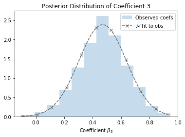
The figure above shows the posterior distribution of one of the coefficients from the SUSY data set¹, which we’ll be using throughout this essay. A maximum likelihood estimate of the coefficient would come out to around 0.47, but look at 0.4 or even 0.6 — they seem pretty promising too! It’s easy to see that, given the variance of this coefficient, different samplings of the training set might give rise to very different maximum likelihood estimates. In fact, being armed with the coefficient distribution opens up a number of possibilities:

• Feature selection via significance tests. How confident am I that the coefficient is actually nonzero?
• Bayesian prediction. Produce a prediction by combining the predictions of multiple models, weighted by probability.
• Iterative regression. Train follow-on models using the current model as a prior.
• Explore / exploit. For example, with Thompson sampling, we can sample a model from the distribution for each query to incorporate random exploration into inference.

But how do we compute the distribution? In the case of linear regression, there’s a closed-form solution for coefficient variance. But logistic regression has no such easy answer, since its coefficients are not necessarily normally distributed. In practice, there are two basic approaches: bootstrapping and Laplace approximation. In bootstrapping we sample $n$ different training sets with replacement, train a model with each one, and compute summary statistics (i.e. $\hat{\mu }=\frac{{\sum }_i^n{\beta }_i}{n-1}$ and $\hat{\sigma }=\frac{\sigma }{\sqrt{n}}$) to estimate a Gaussian $\mathcal{N}(\hat{\mu },{\hat{\sigma }}^2)$ for the resulting coefficients. “A Gaussian?” you might ask, “But I thought you said the coefficients aren’t necessarily normally distributed!” This is true, but in a typical real-world training scenario, there are enough training examples being added into the log-likelihood that the distribution becomes roughly Gaussian on account of the central limit theorem. Hence a Gaussian is a reasonable choice for approximating the distribution. Bootstrapping is the approach we’ve taken for generating the baseline charts in this essay. It produces a very robust estimate of the distribution, but it can also be very expensive, since it requires sampling the dataset many times (potentially hundreds of times) and training a model each time.

The Laplace approximation is a far less computationally intensive approach. You might have heard that once training is complete, you can invert the negative second derivative or Hessian of the log-likelihood for an approximate covariance matrix of the coefficients. This is a curious and remarkable fact: what has the Hessian got to with the posterior distribution of coefficients, and why does inverting it approximate the distribution? How are they connected? Providing an intuitively satisfying answer to this question, and a few others along the way, is the goal of this essay.

Background: The Taylor Series

The Taylor series, perhaps the most useful approximation tool in science and engineering, is shown below.

$$f(a)+\frac{f^{\prime }(a)}{1!}(x-a)+\frac{f^{\prime \prime }(a)}{2!}(x-a{)}^2+\frac{f^{\prime \prime \prime }(a)}{3!}(x-a{)}^3+\dots$$

In a nutshell, suppose we want to compute some function $f(x)$, but it’s very complicated and difficult to compute. We can get an approximate answer by computing a simpler function: an $n$-degree polynomial fit to function $f(x)$ by aligning their derivatives at some point $a$. For example, suppose we choose point $a=0$ and use a second-order Taylor approximation of $f(x)$. The approximation would be defined as follows:

$$f(x)\approx A(x)=f(0)+f^{\prime }(0)x+\frac{f^{\prime \prime }(0)}{2}{x}^2$$

At $x=0$, the approximation evaluates to:

$$\begin{array}{rl}A(0)& =f(0)+f^{\prime }(0)\cdot 0+\frac{f^{\prime \prime }(0)}{2}\cdot 0^2\\ & =f(0)+0+0\\ & =f(0)\end{array}$$

The derivative of the approximation would be:

$$\begin{array}{rl}{A}^{\prime }(0)& =0+f^{\prime }(0)+2\cdot \frac{f^{\prime \prime }(0)}{2}x\\ & =f^{\prime }(0)+f^{\prime \prime }(0)\cdot 0\\ & =f^{\prime }(0)\end{array}$$

And the second derivative:

$$\begin{array}{rl}{A}^{\prime \prime }(0)& =0+1\cdot f^{\prime \prime }(0)\\ & =f^{\prime \prime }(0)\end{array}$$

In other words, if we take the first and second derivative of the approximation, we arrive at the first and second derivative of the original function, respectively. We can customize how closely the shape of the polynomial matches the shape of the original function at the given point by choosing the number of terms in the polynomial. How closely the approximation matches the original function at any distance from this point depends on the nature of the function, but in practice, a second-order polynomial is usually enough, given a reasonable amount of locality around the point.

This approximation is very useful in a computational context because polynomials are relatively easy to compute, we can choose the number of terms in the polynomial to trade off computation time versus accuracy, and we can approximate any function for which we can compute derivates at the same point.

Approximating Likelihood

Let’s revisit the logistic likelihood function now, and see how the Taylor series might apply. Recall the log-likelihood for logistic regression:

$$\ln \mathcal{L}(x)=\sum _{i=1}^n{y}_i\ln g(x_i^{\top }\beta )+(1-y_i)\ln (1-g(x_i^{\top }\beta ))$$

We can approximate this with a second-order Taylor polynomial as follows.

$$\ln \mathcal{L}(x)\approx \ln \mathcal{L}(a)+\frac{d\ln \mathcal{L}}{d\beta }(a)\cdot (x-a)+\frac{1}{2}\frac{d^2\ln \mathcal{L}}{d{\beta }^2}(a)\cdot (x-a{)}^2$$

At the mode of the posterior distribution, the first derivative is zero since it’s a maximum of the function, hence we can drop the first derivative term from the approximation.

$$\ln \mathcal{L}(x)\approx \ln \mathcal{L}(a)+\frac{1}{2}\frac{d^2\ln \mathcal{L}}{d{\beta }^2}(a)\cdot (x-a{)}^2$$

We can simplify this further by introducing a variable for the second derivative of the log loss function.

$$h=-\frac{d^2\ln \mathcal{L}}{d{\beta }^2}(a)$$ $$\ln \mathcal{L}(x)\approx \ln \mathcal{L}(a)-\frac{h}{2}(x-a{)}^2$$ $$\begin{array}{rl}\mathcal{L}(x)& \approx \exp \{\ln \mathcal{L}(a)-\frac{h}{2}(x-a{)}^2\}\\ & \approx \mathcal{L}(a)\exp \{-\frac{h}{2}(x-a{)}^2\}\end{array}$$

In the last step, we exponentiate both sides and arrive at an approximation that’s proportional to a Gaussian. If we scale the function so that it sums to 1 and represents a probability distribution, we have arrived at a Gaussian with mean $a$ and precision $h$ or variance $h^{-1}$.

$$\mathcal{L}(x)\approx \left(\frac{h}{2\pi }{)}^{\frac{1}{2}}\exp \right\{-\frac{h}{2}(x-a{)}^2\}$$

We can extend this to a $k$-dimensional multivariate space as follows.

$$\begin{array}{rl}\mathcal{L}(x)& \approx \left(\frac{|H|}{(2\pi {)}^k}{)}^{\frac{1}{2}}\exp \right\{-\frac{1}{2}(x-a{)}^{\top }H(x-a)\}\\ & \approx \mathcal{N}(x|a,H^{-1})\end{array}$$

Hence the posterior likelihood distribution can be approximated by a second-order Taylor expansion by way of a Gaussian with mean $a$ and covariance matrix $H^{-1}$. This is an instance of the Laplace approximation, where we approximate a posterior distribution with a Gaussian centered at the maximum a posteriori estimate.

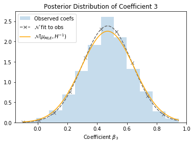
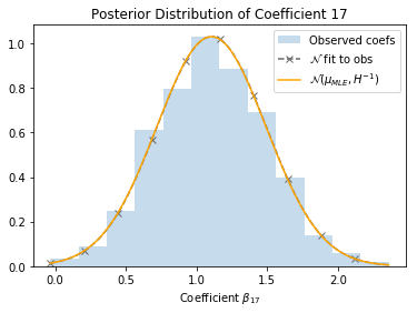
Let’s return to the SUSY dataset, and see how this applies in practice. The dashed line represents a Gaussian fit directly to the observed coefficients, and the orange line represents the Gaussian estimated from the Hessian. They’re pretty close!

Future Topics

• Large features spaces
• Binary features

Footnotes

1. Baldi, P., P. Sadowski, and D. Whiteson. “Searching for Exotic Particles in High-energy Physics with Deep Learning.” Nature Communications 5 (July 2, 2014) https://archive.ics.uci.edu/ml/datasets/SUSY ↩