Learning to Rank with Linear Models

Most active research and applications of learning to rank algorithms focus on nonlinear modeling techniques like SVMs and boosted decision trees. There are, however, very natural ways to model ranking problems with simple linear models. In this note we’ll explore how linear models like logistic regression can be extended to natively support learning to rank objectives. The benefits would be twofold:

1. Linear models are easier to inspect, explain, debug, and deploy than nonlinear models.
2. Linear models are still in wide use in settings where large scale prohibits deploying more sophisticated models. A learning to rank objective could provide a boost for projects already using linear models for ranking problems.

Background

The learning to rank problem can be stated as follows: given a query (e.g. user entry into a search engine), and a set of matching results (e.g. a list of urls matching the search), find an ordering of the results that places more relevant results higher in the list and less relevant results lower. Ranking problems differ from typical supervised learning problems in that they partition the observations into query groups.

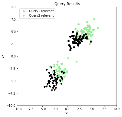
Figure 1. Results from two different queries

In Figure 1, we have a synthesized dataset containing search results for two queries, very creatively named Query1 and Query2. The result documents have been placed in a feature space of two dimensions, and to keep things simple, we’ve limited them to binary labels: a result is either relevant or it’s not. This can be extended to handle labels of varying degrees of relevance without much trouble.

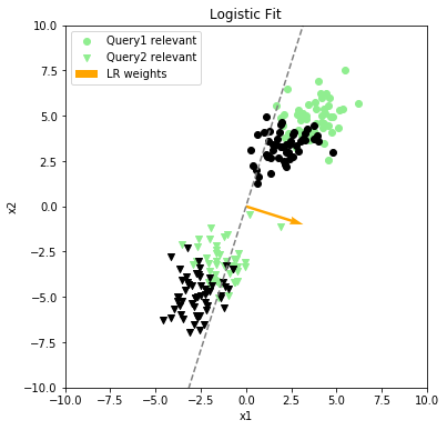
At this point, it might be tempting to model this as an ordinary classification problem, and use a model like logistic regression to predict a relevance probability for each document. Figure 2 below illustrates how doing so can go wrong.

Figure 2. A logistic regression model fit to the data.

In this case, the documents for both queries share a clear linear correlation between the document features and relevance response, but logistic regression fails to find it because of a small difference in the feature distributions between the two queries. The plot on the right side of Figure 2 shows the Query2 documents projected onto the learned weights, where the scores are ordered high to low. While there is some general tendency to rank relevant documents higher, the results are overall very mixed. Many relevant results appear quite low in the list, and many irrelevant results have higher scores.

Pairwise Ranking

In ¹ it was shown that, for linear models, the learning to rank problem can be transformed into an ordinary classification problem by modeling the differences between pairs of results rather than modeling the results directly. The intuition for this is that if we model the probability that any two results are ordered correctly within a query group, we neatly side-step any problems with differing distributions between query groups. The probability pij that result i should be ranked ahead of result j can be expressed as follows²:

$$p_{ij}=\frac{1}{1+\exp (-(s_i-s_j))}$$

Where $s_i=x_i^{\mathsf{T}}w$, $x_i$ the feature vector for result $i$, and $w$ is the weight vector. This is equivalent to an ordinary logistic regression model where the feature vectors have been subtracted ahead of time:

$$\begin{array}{rl}{s}_i-s_j& =x_i^{\mathsf{T}}w-x_j^{\mathsf{T}}w\\ & =(x_i-x_j{)}^{\mathsf{T}}w\end{array}$$

Hence we can transform a learning to rank problem into an ordinary classification problem by applying the following operations to the training set as a pre-processing step:

• Group training examples by query
• Within each group, choose pairs of examples whose labels disagree
• For each pair of feature vectors and labels ($x_i$, $y_i$), ($x_j$, $y_j$) generate a transformed training example ($x_i-x_j$, $1(y_i>y_j)$).

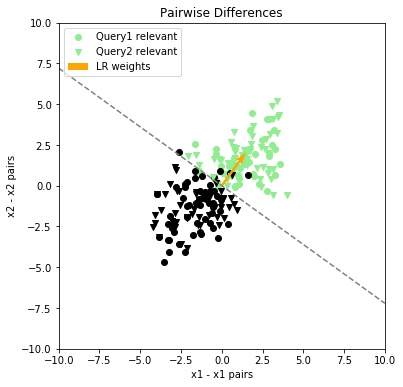
Figure 3 shows the results of applying this transformation to the dataset from Figure 1.

Figure 3. The transformed pairwise difference data, with learned logistic weight vector

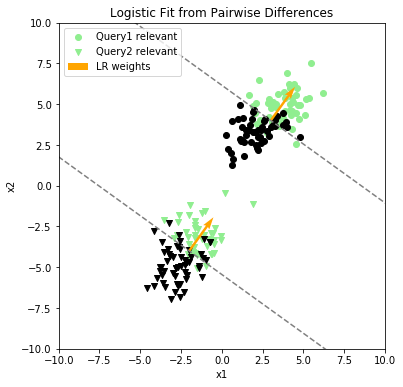
In this transformed problem, logistic regression finds the correlation. Figure 4 below shows the results of applying the new model to the original dataset. It’s easy to see that this model does a much better job discriminating between relevant and irrelevant results, and the projection of results onto the new weight vector is clearly superior: with a few minor exceptions around the middle of the range, relevant results are ranked ahead of irrelevant results.

The last figure illustrates a couple important points about pairwise ranking models:

• The learned function is a pairwise function $f(x_i-x_j)$, but the scoring function is a point-wise function $f(x_i)$. Since our goal is to find an overall ordering of results within a group, we don’t need to bother with producing probability estimates of orderings between individual pairs of results. Hence it’s sufficient to project each point within a group onto the weights individually and use the resulting raw score as a sort key.
• Rankings are valid only within query groups. Notice that if the results of both queries were to be projected onto the weight vector at the same time, the irrelevant results for Query1 would rank ahead of the relevant results for Query2. This is clearly a nonsensical result, so one must be careful not to compare scores between groups.

LambdaRank

The main observation of LambdaRank is that when optimizing, we’re concerned with the gradient of the cost function rather than the cost function itself, and this gradient can be shaped to produce a result that optimizes for a desired validation metric along with minimizing the cost of ranking inversions². For example, we can imagine that there is some cost function C whose gradient includes a scaling factor that “pulls” the model in a direction that also maximizes the (non-smooth) NDCG ranking metric:

$$\begin{array}{rl}{\lambda }_{ij}& =\frac{\partial C(s_i-s_j)}{\partial s_i}\\ & =\frac{-1}{1+\exp (s_i-s_j)}|{\Delta }_{NDCG}|\end{array}$$

It’s not important that we recover the actual cost function C corresponding to this gradient , since we need only the gradient. It’s been shown empirically that this formulation produces better results than simple pairwise ranking, and actually optimizes the NDCG metric directly². NDCG would typically be difficult to optimize directly since it’s discontinuous, but the LambdaRank formulation allows us to side-step this difficulty by computing the full metric on the list of results at each gradient step. Specifically, we compute the metric twice — once with results i and j in their predicted order and again with their positions flipped — and use the absolute difference to scale the gradient.

Code

The jupyter notebook used to generate the plots in this note can be found here.

Footnotes

1. Herbrich, R. (1999). Support vector learning for ordinal regression. In 9th International Conference on Artificial Neural Networks: ICANN ’99 (Vol. 1999, pp. 97–102). IEE. https://doi.org/10.1049/cp:19991091 ↩

2. Burges, Christopher J.C., From RankNet to LambdaRank to LambdaMART: An Overview, Microsoft Research Technical Report MSR-TR-2010-82, 2010, https://www.microsoft.com/en-us/research/wp-content/uploads/2016/02/MSR-TR-2010-82.pdf ↩ ↩² ↩³